Composing a processing sequence

The xdas library provides various routines from NumPy, SciPy, and ObsPy that have been optimized for DAS DataArray objects, and which can be incorporated in a processing pipeline. See Processing larger-than-memory data for an explanation of the xdas processing workflows, e.g. for bigger-than-RAM datasets. Higher-level operations (FK-filters, STA/LTA detector, etc.) can be constructed from a sequence of the elementary operations implemented in xdas. To facilitate this and other user-defined operations, xdas offers a convenient framework to create and execute a (nested) sequences of atomic operations. By using sequences, built-in and user-defined processing tasks mesh seamlessly with the optimization and IO-infrastructure that xdas offers, improving the robustness and reproducibility of complex processing pipelines.

Chaining elementary operations (atoms)

There are three “flavours” declaring the atoms that can be used to compose a sequence, illustrated by the following example:

import numpy as np
import xdas
import xdas.signal as xs
from xdas.atoms import Partial, Sequential, IIRFilter

sequence = Sequential(
    [
      xs.taper(..., dim="time"),
      Partial(np.square),
      IIRFilter(order=4, cutoff=1.5, btype="highpass", dim="time"),
    ]
)
sequence

Sequence:
  0: taper(..., dim=time)
  1: square(...)
  2: 
    IIRFilter(order=4, cutoff=1.5, btype=highpass, ftype=butter, stype=sos, dim=time)

In the snippet above, we define our sequence as an instance of the Sequential class, which contains three operations. The first operation applies a Tukey taper along the time dimension, encoded by the xdas implementation of the SciPy library routines (xdas.signal). Since this functions takes a data array as the first argument, we use ... as a placeholder.

The second operation in this sequence is defined by the square operation built into NumPy. Since this function is not imported directly from xdas, using ... as a placeholder won’t work. This is where Partial comes in: wrapping Partial around np.square would be equivalent to np.square(...), effectively converting an arbitrary routine into an xdas routine and inserting a placeholder as the first argument (to be substituted with a data array later).

The last operation, IIRFilter, instantiates a specific class dedicated to chunked execution. It inherits from the Atom class, which handles the logic of initialising and passing around state objects (like the filter state). This allows us to process our data one chunk at a time, without explicitly having to handle state updates and transfer.

Executing a sequence

Once the processing sequence has been defined, it can operate on data in memory by simply calling the sequence with the data array as the argument:

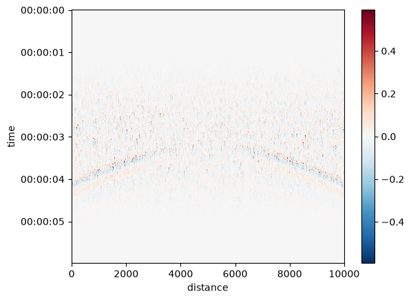
from xdas.synthetics import wavelet_wavefronts

da = wavelet_wavefronts()
result = sequence(da)
result.plot(yincrease=False)

The same sequence can be re-used, so it only needs to be defined once.

For executing a sequence on chunked data (e.g., larger-than-memory data sets), see the next section: Processing larger-than-memory data.

Defining custom atoms

The Partial method is a convenient wrapper for simple functions that take an xdas DataArray as the first argument, which covers a lot of cases. However, more complex routines, particularly those that rely on a state, will require a more explicit treatment. Such operations can be subclassed from the Atom base class, and adhere to the following structure:

from xdas.atoms import Atom, State

class MyStatefulRoutine(Atom):

  def __init__(self, a, b, c=10):
    super().__init__()
    # Set class-specific parameters
    self.a = a
    self.b = b
    self.c = c
    # Define the state variable (if needed)
    self.state = State(...)

  def initialize(self, da, **kwargs):
    # Initialize state based on DataArray ``da``
    ...
  
  def call(self, da, **kwargs):
    # Apply routine to DataArray ``da``
    ...