Working with Large-N Seismic Arrays

The virtualization capabilities of Xdas make it a good candidate for working with the large datasets produced by large-N seismic arrays.

In this section, we will present several examples of how to handle long and numerous time series.

Note

This part encourages experimenting with seismic data. Depending on the most common use cases users find, this could lead to changes in development direction.

Exploring a dataset

We will start by exploring a synthetic dataset composed of 7 stations, each with 3 channels (HHZ, HHN, HHE). Each trace for each station and channel is stored in multiple one-minute-long files. Some files are missing, resulting in data gaps. The sampling rate is 100 Hz. The data is organized in a directory structure that groups files by station.

To open the dataset, we will provide a pattern that describes the directory structure and file names to the xdas.open function. The pattern is a string containing placeholders for the network, station, location, channel, start time, and end time. Placeholders for named fields are enclosed in curly braces, while simple brackets are used for varying parts of the file name that will be concatenated into different acquisitions (meant for changes in acquisition parameters).

Next, we will plot the availability of the dataset.

import xdas as xd

pattern = "NX/{station}/NX.{station}.00.{channel}__[acquisition].mseed"
dc = xd.open(pattern, engine="miniseed")
xd.plot_availability(dc, dim="time")

We can see that indeed some data is missing. Yet, as often, the different channels are synchronized. We can therefore reorganize the data by concatenating the channels of each station.

dc = xd.DataCollection(
    {
        station: xd.concatenate(objs, dim="channel")
        for station in dc
        for objs in zip(*[dc[station][channel] for channel in dc[station]]) 
    },
    name="station",
)
xd.plot_availability(dc, dim="time")

In our case, all stations are synchronized to GPS time. By selecting a time range where no data is missing, we can concatenate the stations to obtain an N-dimensional array representation of the dataset.

dc = dc.sel(time=slice("2024-01-01T00:01:00", "2024-01-01T00:02:59.99"))
da = xd.concatenate((dc[station] for station in dc), dim="station")
da

<xdas.DataArray (station: 7, channel: 3, time: 12000)>
DaskArray: 1.9MB (float64)
Coordinates:
    network: 'NX'
    location: '00'
  * time (time): 2024-01-01T00:01:00.000 to 2024-01-01T00:02:59.990
  * channel (channel): ['HHE' ... 'HHZ']
  * station (station): ['SX001' ... 'SX007']

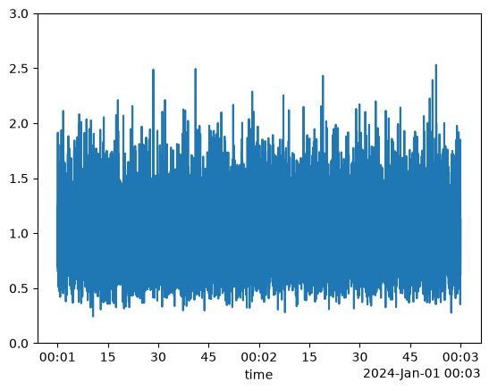
This is useful for performing array analysis. In this example, we simply stack the energy.

trace = np.square(da).mean("channel").mean("station")
trace.plot(ylim=(0, 3))

All the processing capabilities of Xdas can be applied to the dataset. We encourage readers to explore the various possibilities.